Introduction

A Hidden Markov Model, or HMM is a special case of a Bayesian Network.

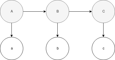
In the Bayesian Network representation above of a first-order HMM, there are three hidden states, and three observations. \(A\), \(B\), and \(C\) form the hidden events, and \(a\), \(b\), and \(c\) form the observations. The above HMM is first-order because the likelihood of each hidden event (except the first), is determined solely by the likelihood of the previous event. The above HMM would be second order if there was a dependency, or arrow pointing from \(A\) to \(C\), as \(C\) is dependent upon \(A\) and \(B\) in that case, as opposed to solely \(B\) in the above graph.

The likelihood for the above graph is simple to compute because of the simple dependency structure. \(P(A,B,C,a,b,c)=P(A)P(a|A)P(B|A)P(b|B)p(C|B)p(c|C)\).

The events \(A\), \(B\), and \(C\) are used to represent latent variables. The events \(a\), \(b\), and \(c\) are used to represent observations.

Modeling

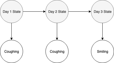
A HMM can be used to model a sequence of events with observations. A common situation is that someone goes to the doctor, and indicates their symptoms. The doctor either determines the patient is sick or healthy, based upon the reported symptoms. This someone goes to the doctor three separate occasions, and this is modeled by the below 1st order HMM.

The above 1st order HMM could be a model for a patient seeing a doctor on three separate occasions. On the first and second visit, the patient was coughing. On the last visit, the patient was smiling. Whether the patient was sick or healthy is unobserved, but a probabilistic argument can be made. We can generally guess that a patient is sick if they are coughing, and healthy if they are not, but it is possible a patient could be coughing when they see a doctor, and not be sick. A patient could not feel well or be sick, but still be smiling and happy.

Let’s explicitly define the possible events for each random variable. For each hidden variable, Day One State, Day Two State, and Day Three State, the patient is either sick or healthy. For each observation, the patient is either coughing or smiling.

Let’s define the probability of Day One State.

State	Likelihood
Healthy	0.80
Sick	0.20

where the first entry indicates the probability that the patient is healthy, 80%, and the second entry indicates the probability that the patient is sick, 20%.

Let’s define the transition probabilities, namely the likelihood of the next hidden state given the current hidden state.

	Healthy	Sick
Healthy	0.90	0.10
Sick	0.50	0.50

The rows indicate the current state, and the columns indicate the next state. For example, the probability of becoming sick if the patient is healthy is 10%.

Let’s define the emission probabilities, namely the probability that coughing or smiling is observed from the patient.

	Smiling	Coughing
Healthy	0.75	0.25
Sick	0.40	0.60

For example, the probability that the patient would be coughing if he or she is sick is 60%.

With the probabilities defined, we can compute likelihoods for the model.

Likelihoods

The joint probability distribution for a 1st order HMM in general with states \(z_i\) and observations \(x_j\) is

\[P(x_1,...,x_T,z_1,...,z_t)=P(z_1)\prod_{t=1}^{T-1}P(z_{t+1}|z_t)\prod_{t=1}^TP(x_t|z_t)\]

The joint probability distribution for our model is

\[P(A,B,C,a,b,c)=P(A)P(a|A)P(B|A)P(b|B)P(C|B)P(c|C)\]

Given a sequence of observations, namely “Coughing”, “Coughing”, and “Smiling”, we can identify the most likely sequence of states, by identifying the sequence of states that maximizes the joint probability distribution. A trivial approach is to enumerate all possible hidden states and then choose the hidden states with the highest likelihood. This is an \(O(|S|^T)\) approach, where \(S\) is a set containing all possible states.

Viterbi Algorithm

The Viterbi Algorithm is a dynamic programming approach to identify the most likely sequence of hidden states of a first order HMM. Intuitively, the Viterbi Algorithm at each step \(i\) identifies the most likely sequence of the hidden states of length \(i\).

Derivation

Consider the joint probability distribution for a 1st order HMM,

\[P(x_1,...,x_T,z_1,...,z_t)=P(z_1)\prod_{t=1}^{T-1}P(z_{t+1}|z_t)\prod_{t=1}^TP(x_t|z_t)\]

We can simplify this by defining \(P(z_{1}|z_{0})=P(z_1)\), substituting and rewriting bounds,

\[P(x_1,...,x_T,z_1,...,z_t)=\prod_{t=1}^{T}P(z_{t}|z_{t-1})P(x_t|z_t)\]

Let’s define

\[r(z_1,...,z_k)=\prod_{t=1}^{T}P(z_{t}|z_{t-1})P(x_t|z_t)\]

Consider function \(\Psi(k,v)\). \(\Psi\) represents the probability that the hidden state sequence of \(k\) observations ends in hidden state \(v\). Let \(S(k,v)\) be the set of all sequences of length \(k\) that end in \(v\).

In general,

\[\begin{align} \Psi(k,v)=&\max_{S(k,v)}\,r(z_1,...,z_k=v)\\ =&max_{z_1,...,z_{k-1},z_k=v}\prod_{t=1}^kP(z_{t}|z_{t-1})P(x_t|z_t)\\ =&max_{z_1,...,z_{k-1},z_k=v}P(v|z_{k-1})P(x_k|v)\prod_{t=1}^{k-1}P(z_{t}|z_{t-1})P(x_t|z_t)\\ =&max_{u\in H}\,\Psi(k-1,u)P(v|u)P(x_k|v) \end{align}\]

Application

In the first step, the most likely hidden state for \(A\) is computed, namely “Healthy”, since the probability that “Coughing” will be observed is higher if the hidden state is “Healthy” as opposed to “Sick”. Namely, \(0.80\times0.25>0.20\times0.60\). Intuitively, this means that it is more likely (for this model) that a person was actually healthy, but happened to be coughing at their appointment.

In the second step, the most likely hidden state for \(B\) is computed. The probability that the patient remains healthy at the second observation is \(0.80\times0.25\times0.90\), which is the probability that the patient is healthy, coughing was observed, and was still healthy at the second observation. The probability that coughing was observed a second time for the above situation is \(0.80\times0.25\times0.90\times0.25\). The probability that the patient becomes sick at the second observation is \(0.20\times0.60\times 0.10\), which is the probability that the patient was healthy, emitted coughing at the first observation, and then became sick. The probability that coughing is observed a second time for this assignment of values is \(0.20\times0.60\times0.10\times0.60\).

Thus, because \(0.80\times0.25\times0.90\times0.25>0.20\times0.60\times0.10\times0.60\), the most likely sequence of states for the first two days is “Healthy”, and “Healthy”.

In the third step, \(0.80\times0.25\times0.90\times0.25\times0.90\times0.75\), the probability that the patient remained healthy, and was smiling, is compared with \(0.80\times0.25\times0.90\times0.25\times0.10\times0.40\). The patient remaining healthy has a higher probability than the patient became sick and was still smiling, thus the most likely sequence of hidden states is “Healthy”, “Healthy”, “Healthy”.

Sources

EECS 445 Lecture

Contact

Please feel free to email me at cody@codymorterud.com with any questions or concerns. Thanks!